


A radar transmitter has emitted a beam of radar waves. For a moment, let us imagine that these radar waves, or radar pulse, behaves like a bouncy ball, where it bounces off an object on the Earth’s surface and then bounces back up to the transmitter.
Now let’s imagine that these pulses rain down on earth like millions of rubber balls, but when they come in contact with an object, they retain some information about that object in the form of electromagnetic waves. Now we can analyze and extrapolate the data the bounce returned and understand more about what the ball bounced off.
Interpreting and visualizing information from a radar image is dependent on understanding the bounce-mechanism – or how the radar pulse interacts with the target. The intensity and polarization of data – the information carried with the ball back to the transmitter, also known as backscatter – is determined by several factors.
This image shows all possible bounce-mechanisms. Each bounce type returns with distinctive data:
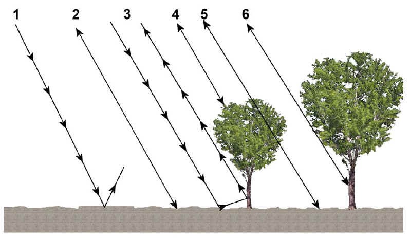
Model showing all possible bounce mechanisms, or responses of electromagnetic waves to materials they cannot pass through.
Bounce Type 1
The radar signal bounces off a smooth, flat surface and does not return to the sensor. In the radar image this is represented as very dark pixels. This bounce type is called “specular reflection.” Specular reflection is why anything smooth and flat – like calm water bodies, roads, and parking lots – are visually dark in radar images. Users can delineate specular reflection into functional visual data through the Level Slice tool in Radar Analyst Workstation in ERDAS IMAGINE.
Bounce Type 2
The radar signal bounces off a rough, flat surface and scatters in every direction with only a few data points bouncing back to the sensor. The orientation of each radar pulse results in various shades of grey pixels in the radar image.
Bounce Type 3
A very common return is the double-bounce. Here we see the signal bounce off one solid surface (the ground), and then off of another (the tree). A double-bounce tends to return a strong signal and results in very bright pixels in the radar image.
However, none of this is very descriptive information. A road alongside a building or the side of a ship at sea will also return the same strong double-bounce. By understanding the context of the image as well as bounce mechanisms, we can better understand what features the pixels represent in a radar image.
For example, is this return from a road or a bridge? A car or a ship? It is important to know what type of radar image you are viewing before you can begin to interpret the data.
This return also makes us take another factor into account: look direction. The look direction, or the direction in which the pulse was emitted towards the Earth’s surface can affect the returns as well. Take the following image, for example:
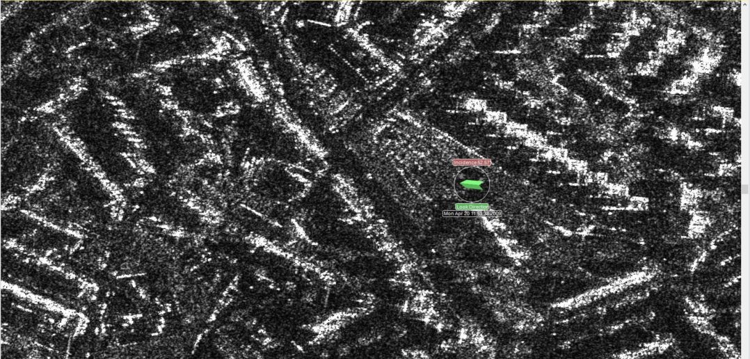
A city image captured using radar bounce mechanisms with radar beam looking East to West.
When it captured this image of the city, the radar beam was looking East to West. The dark line running diagonally, top to bottom in the center of the image is a main road. The smooth, flat road results in a specular reflection, making the road look very dark.
Then, the reflected signal hits buildings running along the west side of the road creating a double-bounce interaction. Because of the intensity of the double-bounce mechanism, those pixels appear to be very light. There are certainly buildings on the east side of the road, and they are every bit as substantial as the buildings on the west side. But because the pulse went from east to west, as indicated by the look direction arrow, there is no possibility of a double-bounce from the buildings on the east side of the road, and they will never appear as brightly in the image.
Bounce Type 4
The top-of-canopy scatter occurs when the radar signal is returned from the first surface encountered without penetrating to the ground. This is highly dependent on the length of the radar wave you are examining. When you are dealing with short radar wavelengths, such as X-band radar, this is the expected return and is equivalent to the first-return from a LIDAR sensor. When you are dealing with radar with longer wavelengths, however, you may not ever get a top-of-canopy return.
Bounce Type 5
There are various ways to determine how bounce mechanisms are used to interpret and even classify a radar image. For example, we know if a radar transmitted the beams in a vertical (the waves emanated in an up-and-down orientation) or horizontal (the waves went side-to-side) direction. We can then sense how the waves were oriented when they returned to the sensor – were they in the same orientation, or did they rotate? Then we can use Polarimetric Classification algorithms, an option in the Radar Utilities in ERDAS IMAGINE, to detect the various polarimetric bands and deduce the operant bounce mechanism for each pixel.
There are various ways to determine how bounce mechanisms are used to interpret and even classify a radar image. For example, we know if a radar transmitted the beams in a vertical (the waves emanated in an up-and-down orientation) or horizontal (the waves went side-to-side) direction. We can then sense how the waves were oriented when they returned to the sensor – were they in the same orientation, or did they rotate? Then we can use Polarimetric Classification algorithms, an option in the Radar Utilities in ERDAS IMAGINE, to detect the various polarimetric bands and deduce the operant bounce mechanism for each pixel.
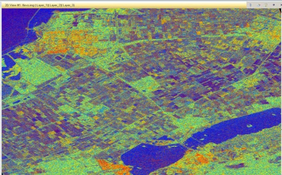
A classification of a quad-pole Radarsat-2 scene of Flevoland, Holland. The Polarimetric Classification Tool has classified the scene into three classes based on deduced bounce mechanisms.
Bounce Type 6
The beam bounces off an elevated target and returns to the sensor. Because the target is elevated, the travel time for the radar beam to hit its target and return is much shorter. This can cause a “distortion,” or a spatial displacement, of the feature.
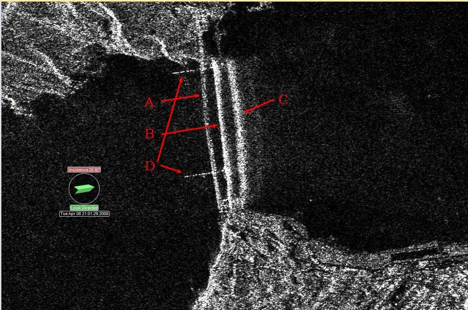
TerraSAR-X Image of the Golden Gate Bridge in San Francisco, California.
Let’s look at an extreme case of spatial displacement by examining a radar image of the Golden Gate Bridge in San Francisco, California.
This image is difficult to understand due to several simultaneous bounce mechanisms. To begin interpreting this image, you must first understand that the look direction is West to East indicated by the green arrow of the Look Direction tool.
A depicts a direct specular reflection, or one bounce off the bridge. Note that the dark pixels continue off the bridge and onto the road as it passes onto land in the North (Marin County).
B depicts a double bounce – first bouncing off the bridge, then the water, and finally returning to the sensor.
C depicts a triple bounce – first bouncing on the water, then the underside of the bridge, then bouncing off the water a second time and returning to the sensor.
Bounces for both B and C have longer paths to travel, thus taking more time to return and resulting in time data displacement.
D is bouncing off the bridge’s towers. Contrary to B and C, the towers are tall, so the beam takes less time to bounce off the tower and return to the sensor, causing higher sections of the towers to be displaced and appear to lean toward the sensor. This phenomenon, known as “layover” can be common in images.
Once you understand how bounce mechanisms affect a radar image, it becomes easier to interpret features that the image is displaying. Sure, it takes a lot of practice and hard work to become skilled at interpreting radar images, but you have to start somewhere. Just follow the bouncing ball!